concept
Multiple alignment of RNA sequence data according to structure uses the criterion of covariation as a means to delimit stems, loops, and regions of alignment-ambiguity. Every region delimited according to this method is defendable across all taxa, and as such the final alignment can be seen as a model for the evolution of the molecule in question. Regions that cannot be aligned across all taxa with 100 percent confidence, using the same criterion for all taxa, are explicitly excluded from primary homology statements. As such, this method can be seen as very conservative relative to algorithm-based alignments, for which no biological criteria exist for assigning positional nucleotide homology in RNA datasets.
For all alignments listed on jRNA, the following methodology was used. Sequences were aligned manually according to secondary structure, with the notation following Kjer et al. (1994) and Kjer (1995), with slight modifications (see Gillespie et al. 2004b). Alignment initially followed the secondary structural models of Gutell et al. (1994), which were obtained from the Comparative RNA Website (Cannone et al., 2002), and was further modified according to an existing chrysomelid D2 model (Gillespie et al., 2003, 2004a) and a trichopteran D3 model (Kjer et al. 2001). Individual sequences, especially hairpin-stem loops, were evaluated in the program mfold version 3.1, which folds rRNA based on free energy minimization (Matthews et al., 1999; Zuker et al., 1999). These free energy-based predictions were used to facilitate the search for potential base-pairing stems, which were confirmed only by the presence of compensatory base changes across all taxa. Regions in which positional homology assessments were ambiguous across all taxa were defined according to structural criteria as in Kjer (1997), and described as regions of alignment ambiguity (RAA) or regions of slipped-strand compensation (RSC; Levinson & Gutman, 1987; for reviews regarding rRNA sequence alignment see Schultes et al., 1999; Hancock & Vogler, 2000). Briefly, ambiguous regions in which base-pairing was not identifiable were characterized as RAAs. For ambiguous regions wherein base-pairing was observed (RSCs), compensatory base change evidence was used to confirm structures that were not consistent across the alignment due to the high occurrence of unknown insertion and deletion events (indels). For some ambiguous regions in the alignment caused by the expanding and contracting of hairpin stem-loops, RSCs were further characterized as RECs (regions of expansion and contraction) based on structural evidence used to identify separate non-pairing ambiguous regions of the alignment (terminal bulges). A recent paper addresses the characterization of RAAs, RSCs and RECs with a discussion on phylogenetic methods accommodating these regions (Gillespie 2004).
method
While various text editors can be used, the process of structural alignment is greatly facilitated while performed in a platform that allows for underlining and coloration of basepairs, as well as manipulation of entire blocks of the alignment (i.e., moving portions of the alignment to different interleaved blocks, adding structural notation such as brackets ([ ]) and bars (| |) and recoding ambiguously aligned regions). In our laboratories, edited sequences are exported to the program SeAl and broken into conserved blocks based on published secondary structural models. These blocks are then entered into Microsoft Word ™ and aligned according to the method described in Kjer (1995). Breaking the alignment into blocks facilitates the visualization of compensatory base changes (positional covariation) in long-range helices. It also provides subsets of the data (localized structural motifs within the molecule) that are easier to import into folding programs, such as mfold, and thus do not require constraints to be included into folding algorithms.
The process of structural alignment is outlined below in a simple example:
1
Begin with unaligned sequence data that is left justified.

2
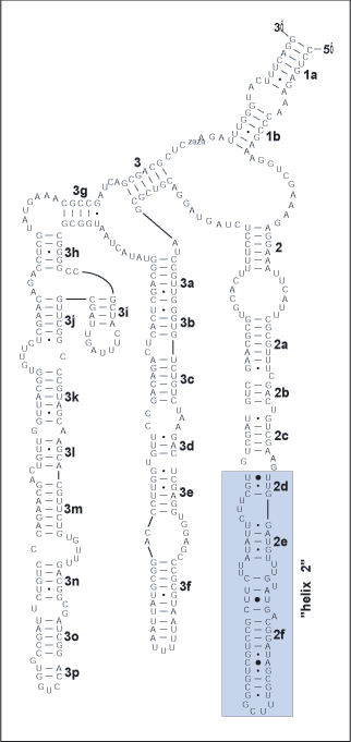
Search on public databases for a published structure for this sequence region. For example, the above is a section of helix 2 of expansion segment D2 of the 28S rRNA from Gillespie et al. (2004b). Note: if the closest published structure is phylogenetically distant from the taxa in the alignment, it may be necessary to explore available folding algorithms, for example mfold, for novel/putative helical regions. However, keep in mind that folding algorithms often do not predict accurate structures in RNA molecules, and that sub-optimal predicted structures can often be better estimates than optimal ones (as verified across multiple taxa). Thus, when using folding programs, it is important to verify predicted structures across an alignment by searching for compensatory base changes (CBCs) across helices predicted by the folding algorithms. The primary information we will be using to align the data is biological, as it is derived from evidence of Watson-Crick pairings, GU intermediates, and rare non-canonical pairings. When these pairings are compared across taxa, evidence of CBC may emerge. Every homology hypothesis is supported by either CBC evidence or invariance in unambiguously aligned single stranded regions or helices wherein covariation exists when compared at higher divergence levels. Helices wherein CBC evidence is weak or lacking can be verified as biological structures by consulting multiple sequence alignments across taxa with higher divergences, such as those posted on the Comparative RNA Website. |
 |
3
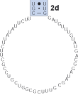
Look for the first helix, in this case, 2d. In this case UUG from the model can be found in most of our sequences. The complement to UUG can be one of the following: CAA, CAG, CGA, CGG, UAA, UAG, or UGA. Note that the ability for GU and UG pairings increases the potential number of basepair combinations in RNA molecules. Searching forward in the sequences for any of these motifs, potential complements are sought to define a putative 2d helix in the alignment.
Delimit complementary strands with bars (||) and leave spaces between your blocks (this is important for subsequent scripted manipulation). Underline nucleotides within bars that form Watson-Crick base-pairs and GU intermediates. The underlining of putative basepairings provides an initial indication of how much evidence or support there is for your homology assignment. If a given column contains "few" underlined nucleotides you might suspect that your homology hypothesis is in fact not supported (or is so conserved that no basepair covariation is detectable at this level of divergence). Supporting evidence for nucleotide pairings is ultimately provided in basepair frequency tables.


4
Find the next helix, 2e. In this case there is a small region between strands 2e' and 2d' which is variable in length and non-pairing. This region is bracketed ([ ]) out in the alignment.


5
Find the next helix. Below four new blocks are delimited. For each taxon there is evidence of stem pairings in blocks 1 and 3 (underlined nucleotides). However, these pairings are not consistent across taxa and there is minimal CBC evidence, thus these regions are bracketed. Note: each column has some evidence for basepairing for a given taxon, but the pairing is not supported across all taxa or each site. These ambiguously aligned regions are known as regions of [slipped-strand compensation]. Because this pairing is not present in all taxa, the block is bracketed. The identification of base-pairing within this region helps delimit blocks 0 and 2.


6
A third helix, 2f, and a single unpaired nucleotide are defined next from block 2 (above). The bonding of helix 2f isolates the unpaired "A". The double bars (|| ||) define an immediate hairpin-stem loop (the last uninterrupted helix that folds back on itself).


7
After careful examination of the final unaligned block we can determine that there are no further helices that can be unambiguously defined. We know at this point that the remaining sequence must represent a hairpin-stem loop that consists of a paired and unpaired region, or terminal bulge. The terminal bulge consists of a minimum of three nucleotides, though it is often comprised of four or more. The terminal bulge is identified via an iterative process, by either examining a sequence from the center outwards, or by identifying pairing regions from the outside regions inwards. Careful use of folding algorithms can often facilitate the characterization of these regions of terminal helix expansion and contraction.


8
Identify the bracketed regions from prior steps wherein hydrogen bonding does not occur. These are regions of ambiguous alignment (RAA). RAAs are bounded by either helices or conserved single stranded regions.


9
Identify the bracketed regions from prior steps wherein hydrogen bonding is inconsistent across columns in the alignment. These are regions of slipped-strand compensation (RSC). RSCs are bounded by either helices or conserved single stranded regions. In this exceptional case the RSC(1) is bounded by RAA(1).


10
Identify the bracketed regions between the conserved hairpin helix and the terminal bulge. These are known as regions of expansion and contraction (REC).


11
Finally, add a pairing mask statement (as used in the program PHASE). This identifies the pairing (evolutionary dependent) and non-pairing (evolutionary independent) regions of the alignment and is important for subsequent scripted manipulations.
